Physics Engine in Odin from Scratch, Part I

25th April 2026 • 22 min read

If you're reading this after completing my series, in which we've built a 3D software renderer in Odin from scratch across 14 parts, then welcome back! In this series, we're going to build a physics engine on top of that. Again, from scratch, and we're going to cover not just the implementation, but all the underlying concepts in depth as well.

Though it's not necessary to go through all the parts of the software renderer series, I highly recommend that you read at least Part I and also Part II and Part III, especially if it's been a while since you've been dealing with linear algebra, specifically with vectors and matrices.

We're going to start with the software renderer project in the state where we left it after the final part, Part XIV. You can download the project in that state from this GitHub repository.

At the end of this series, we'll have a physics engine with raycasting. We'll be able to cast a ray from the position we click on the screen into the virtual world and retrieve the first object the ray hits, if it hits any. We'll use this to push and pull objects under the mouse cursor (LMB to push, RMB to pull).

To ensure our physics engine wouldn't allow objects to penetrate each other, we're going to implement collision resolution (a common feature of physics engines) using two types of colliders: one for rectangular prisms and the other for spheres. For short, we'll call them a box collider and a sphere collider. Thus, we'll have to implement collision resolution between box and box, sphere and sphere, and box and sphere, and you're going to learn about the Separation Axis Theorem (SAT).

We'll be able to "freeze" an object. One such static object will serve us as a floor, since our engine will simulate gravity. Boxes will tip over edges, and spheres will roll as expected. On surfaces tilted above a certain threshold, boxes will start to slide, and spheres will roll naturally. We'll also be able to control how much objects bounce off when they hit another object, and how slippery a surface of an object is by setting their bounciness and friction properties, respectively.

Finally, we'll ensure that when a force is applied to an object that has other objects resting on top, those objects will move as well. (If you would like to use this physics engine to create a Jenga game, you'll have to disable this feature.)

However, we are not going to aim for a physically accurate simulation, but rather for good enough approximations and practical simplifications. A physics simulation we're going to build falls into the category of "game physics", and in the following video, you can see what we'll have by the end of this series.

Such an example of a good enough simplification would be gravity. In reality, by Newton's Law of Universal Gravitation, every two objects with mass attract each other with a force that is directly proportional to the product of their masses and is inversely proportional to the square of the distance between their centers, or simply:

F = G \frac{m_1 m_2}{r^2}

Where F is the gravitational force, G is the gravitational constant, m₁ and m₂ are the masses of the objects, and r is the distance between the centers of the two masses.

That means not only are you attracted to Earth, but Earth is also attracted to you. The force is actually equal in magnitude on both of you, but the effect is very uneven because your mass is tiny compared to Earth's, so Earth's acceleration toward you is imperceptible. You're also attracted to all other objects in the Universe, large or small, near or far; the force is always present, though it becomes extremely weak at large distances. And it's not just you; every object attracts every other object, so the next time someone says, "May the Force be with you," you can reply that the force is literally with everyone and everything all the time, and you'd be right, though possibly at the cost of looking a bit odd.

I apologize for reducing you to an object in the previous paragraph. I did that just for the sake of the example, and you probably already knew all of this and more about Newtonian physics from school. What I really want to say here is that we're not going to implement gravity with this level of accuracy.

The experience with gravity here on Earth is that when you jump, you fall; when you throw a ball up, it goes up for a while and then returns down to Earth, and when you lose your grip while holding a cup of coffee, you'll have to clean up the mess from the floor, not from the ceiling (unless you're in a cramped space, like Harry Potter's cupboard under the stairs). In our physics simulation, we'll focus on this familiar experience. Instead of simulating gravity between all objects, we're going to store gravity as a constant acceleration vector rather than a force.

GRAVITY :: Vector3{0.0, -9.8, 0.0}

Since here on Earth, the gravitational acceleration, the rate at which an object increases speed while falling freely, is approximately 9.8 m/s², and we decided that the upward-pointing vector in our world Cartesian coordinate space is [0, 1, 0].

High-Level Overview

Despite such simplifications, a lot of work still lies ahead of us, but before we start writing any code, let's take a step back and look at the whole project from a bird's-eye view. First, let's talk about how our physics engine fits into the already implemented software renderer.

Data Structures

If you open the model.odinfile, you'll see a definition of the Model struct with a mesh, texture, translation, rotation, scale, and other properties. In this series, we're going to define a couple of new structs, namely RigidBody, BoxCollider, SphereCollider, and Collider union, to extend our Model with.

On top of that, we're also going to define CollisionResult and HitResult to represent the result of collision resolution between objects and between a ray and an object, respectively. We'll come back to these a bit later. Now, let's look at the relationship between the abovementioned structs and union in the following diagram.

classDiagram class Model { mesh: Mesh texture: Texture color: rl.Color wireColor: rl.Color translation: Vector3 rotationMatrix: Matrix4x4 scale: f32 rigidBody: RigidBody collider: Collider } class RigidBody { force: Vector3 velocity: Vector3 torque: Vector3 angularVelocity: Vector3 bounciness: float friction: float isStatic: bool mass: float invMass: float isMovingBySupport: bool } class Collider { <<union>> } class BoxCollider { size: Vector3 } class SphereCollider { radius: float } Model --> RigidBody Model --> Collider Collider <|-- BoxCollider Collider <|-- SphereCollider

If we were building a game engine, I would suggest a different data structure, probably one where we'd have an Entity struct with ID and indices or pointers pointing into contiguous arrays of components (e.g., Transform, Renderer, RigidBody, Collider, etc.), and some Entity Component System. That might actually be a topic for another series of tutorials.

However, we're not building a game engine, and to keep things simple, we're going to treat an existing Model struct as a sort of entity or rather a "game object" (you might be familiar with GameObject from Unity or Actor from Unreal Engine) that, apart from properties related to rendering, will have new properties related to physics simulation.

Core Concept of a Physics Simulation

Before we start adding new structs, let's review what our physics simulation will be responsible for and how it will work in a nutshell. In our software renderer, when we wish to move a selected object, an instance of the Model struct, we pass it by reference to the HandleInputs procedure, where we set the object's translation, rotation, and scale in response to keystrokes.

Further down the main loop, affine transformations are applied to all objects using the ApplyTransformations procedure, where the object's translation, rotation, and scale play a crucial role. After transformations, the objects are taken by the rendering pipeline, whose responsibility is to draw them as viewed from the camera, and eventually lit by our lights, on the screen, and this repeats again and again, frame by frame, as fast as it can.

In this series, instead of directly setting an object's translation and rotation, we're going to modify the HandleInputs procedure to apply force and torque to the object's rigidbody. The physics simulation then uses these properties to update velocity and angularVelocity, and integrates them over time using Euler integration to update the object's translation and rotation. Finally, the simulation also resolves collisions with other objects.

From this point, everything stays the same; affine transformations will be applied, and the objects will go down to the rendering pipeline.

Raycasting

But how do we set in the HandleInputs procedure the force and torque? This is where the concept of raycasting comes into play. As already mentioned at the beginning of this part, we're going to use the mouse to push and pull our object.

Watch the video above again and pay close attention to the position of the cursor. Notice how objects are being pulled as if they were grabbed at the position where the cursor points. Also, notice how the box slightly rotates to the left when it is pulled by the right side.

That's because when a ray hits the object, which illustrates the following image, not just the object is acquired, but also the position where the ray touches the surface, which we're going to call the contact point.

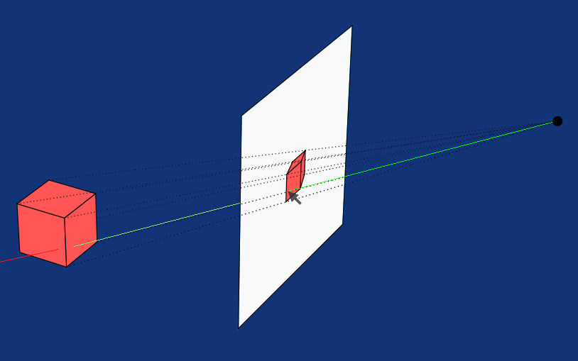
A force in the direction opposite to the ray (in the direction pointing from the contact point to the camera) multiplied by a scalar that effectively sets how fast the object is pulled, is then applied to the object, and torque, which is also multiplied by another scalar, is calculated as the cross product between the vector from the object's center to the contact point and the applied force.

Collision Resolution

Another common responsibility of a physics engine is collision resolution, or to be precise, collision detection and resolution. We don't want to allow two rigid bodies to intersect; when that happens, we push both objects in opposite directions, assuming neither is static, in which case we push only the dynamic one. In the video above, the static object is the biggest cube underneath all the other objects that serves as a floor.

To achieve this, we first need to determine, for each pair of objects, whether they intersect. A naïve approach checks all pairs, which results in quadratic time complexity (O(n²)). There are optimization techniques to address this. We'll return to this later.

There are various techniques for collision detection, each with its own pros and cons. For example, the Gilbert-Johnson-Keerthi (GJK) algorithm can be used to detect collisions between arbitrary convex shapes, but it's a bit more difficult to understand and implement than the Separating Axis Theorem (SAT), especially in 3D.

As we already mentioned, our physics engine will support two types of colliders, sphere colliders and box colliders, and we're going to implement three procedures for detecting collisions between all three combinations of these colliders.

To detect a collision between two boxes, we're going to use SAT. For a box and a sphere, we find the closest point on the box to the sphere's center and compare it with the sphere's radius. Finally, for two spheres, we simply compare the distance between their centers with the sum of their radii. We're going to cover collision detection and resolution, also in more detail, in a dedicated part.

Fixed-Timestep Physics Update

It’s common practice to run physics simulations with a fixed timestep to keep the simulation stable. In our main loop, we let our software renderer run as fast as it can, and we only use deltaTime in the HandleInputs procedure to make translations and rotations frame-time independent.

Our physics update will also run in the main loop, right after HandleInputs, but we won't let it run as fast as possible; instead, we're going to define the PHYSICS_TIMESTEP constant with the value of 1.0 / 60.0. In other words, we want our simulation to run at 60 Hz, meaning it advances the physics simulation in fixed steps of about 16.667 milliseconds. We use this PHYSICS_TIMESTEP constant and deltaTime to wrap our physics simulation in a loop with an accumulator variable like this:

physicsAccumulator += deltaTime
for physicsAccumulator >= PHYSICS_TIMESTEP {
    ApplyPhysics(models, PHYSICS_TIMESTEP)
    ResolveCollisions(models)
    physicsAccumulator -= PHYSICS_TIMESTEP
}

Which brings us to the last part of this high-level overview, and that is a diagram that shows what other procedures are hidden below ApplyPhysics and ResolveCollisions that we're going to implement in the course of this series.

flowchart LR ApplyPhysics --> ApplyGravity ApplyPhysics --> IntegrateLinearForce ApplyPhysics --> IntegrateTorque ApplyGravity --> ApplyFriction ApplyGravity --> ApplyStabilization ApplyGravity --> ApplyTipping ApplyGravity --> ApplyRolling ResolveCollisions --> GetCollisionResult ResolveCollisions --> Correct ResolveCollisions --> MoveStack ResolveCollisions --> Push GetCollisionResult --> BoxBox GetCollisionResult --> BoxSphere GetCollisionResult --> SphereSphere

We're going to implement some other helper procedures along the way as well, such as GetOverhang, FindClosestUpAxis, HasSphereCollider, HasBoxCollider, and several others. I decided to exclude these from the diagram above to keep it nice and simple.

What to Expect in This Series

Last thing before we start writing some code. Similar to Part I of the 3D Software Renderer in Odin from Scratch series, I'd like to briefly describe what's coming in the future parts of this series.

In the next part, I'd like to lay down some foundations, since Part II of the series about software renderer was a very brief math primer, the second part of this series will be a similar physics primer, where we cover the basics of Newtonian physics and numerical integration.

In Part III, we'll get back to coding; we'll set a cornerstore of our simulation as we add a rigidbody, implement gravity, and physics update. At the end of this part, our object will fall once we run the application.

There won't be anything to stop them, though, and we're going to address that in Part IV, where we learn about SAT and implement collision detection and resolution.

In Part V, we're going to add raycasting to be able to push and pull objects under the mouse cursor, and in Part VI, we'll add mass, friction, and bounciness. At this point, our physics simulation will already be quite functional, but one important thing will still be missing, and that is angular motion.

We're going to implement angular motion in Part VII, together with tipping objects over the edge when they overhang, so their center of mass is no longer supported (imagine a book pushed too far off the edge of a table). We'll also implement stabilization; when a box tips over the edge and falls, it lands on the closest face to the ground and stops moving as you'd expect.

At this point, our physics simulation would be complete if we were satisfied with box colliders only, but we'll want to make our simulation more interesting, so in Part VIII, we'll add sphere colliders. Spheres, of course, act differently than boxes; for example, a box might slide, but a sphere usually rolls, so we'll make sure that's the case in our simulation. In this part, we'll also extend our collision resolution procedures to cover cases when a sphere collides with a box and when a sphere collides with another sphere, and our raycasting is also going to need a small update to support sphere colliders.

In the final part, Part IX, we're going to implement stacking. As mentioned already in the introduction, we'll make sure that when a force is applied to an object that has other objects resting on top of it, those objects will move as well, and in the very end, we're going to look at optimizing our simulation with Octress.

If you don't know what Octree is, don't worry about it now; everything will be explained in-depth throughout this series, and you'll gain a lot of knowledge if you've never implemented a physics engine before. To gain knowledge in a fun and interesting way is actually the goal of this series, rather than building something to be used in production.

Preparations

Even though this first part is primarily an introduction to the series, we're going to do some work already. If you want to follow along, and I highly recommend you do so, download from this GitHub repository, if you haven't done so already.

To prepare our software renderer for extension with a physics simulation, we start by adding some helper procedures to the matrix.odin file. First, I'd like to implement a procedure that takes an arbitrary axis and an angle, and returns a rotation matrix. This matrix rotates a vector counterclockwise around the given axis by the specified angle in radians.

MakeRotationMatrixAxisAngle :: proc(axis: Vector3, angle: f32) -> Matrix4x4 {
    a := Vector3Normalize(axis)
    x := a.x
    y := a.y
    z := a.z

    c := math.cos(angle)
    s := math.sin(angle)

    t := 1.0 - c

    return Matrix4x4{
        {t*x*x + c,   t*x*y - s*z, t*x*z + s*y, 0},
        {t*x*y + s*z, t*y*y + c,   t*y*z - s*x, 0},
        {t*x*z - s*y, t*y*z + s*x, t*z*z + c,   0},
        {0,           0,           0,           1},
    }
}

This is also known as Rodrigues' rotation formula, and I'm not going into too much into details, assuming you're already familiar with matrices and transformations. If not, please do read the already recommended Part II and Part III of the software renderer series, where these concepts are explained in more detail.

Another helper procedure I'd like you to add is one for extracting the axes from a rotation matrix. This one is very simple. In our software renderer, we use column-major interpretation for basis vectors, and the X, Y, and Z axes are stored in the first three columns of the matrix.

GetAxesFromRotationMatrix :: proc(mat: Matrix4x4) -> [3]Vector3 {
    return {
        {mat[0][0], mat[1][0], mat[2][0]},
        {mat[0][1], mat[1][1], mat[2][1]},
        {mat[0][2], mat[1][2], mat[2][2]},
    }
}

And the last one, even simpler, for extracting just the Y-axis.

GetUpAxisFromRotationMatrix :: proc(mat: Matrix4x4) -> Vector3 {
    return {
        mat[0][1], mat[1][1], mat[2][1]                   
    }
}

With that done, let's switch over to the model.odin file and in the Model struct definition, replace rotation of type Vector3 with rotationMatrix of type Matrix4x4. The updated struct should look like this:

Model :: struct {
    mesh: Mesh,
    texture: Texture,
    color: rl.Color,
    wireColor: rl.Color,
    translation: Vector3,
    rotationMatrix: Matrix4x4,
    scale: f32,
}

That broke a few things. Let's fix them. First, in the LoadModel procedure, replace the line where we assign Vector3{0.0, 0.0, 0.0} to rotation that no longer exists with this one:

rotationMatrix = MakeRotationMatrix(0,0,0),

Now that we already have a rotation matrix stored with a model, we don't need to make it from rotation in the ApplyTransformation procedure. Hence, from this procedure, remove the line where we define rotationMatrix entirely and change the one where we define modelMatrix, so the updated ApplyTransformation procedure looks like this:

ApplyTransformations :: proc(model: ^Model, camera: Camera) {
    translationMatrix := MakeTranslationMatrix(model.translation.x, model.translation.y, model.translation.z)
    scaleMatrix := MakeScaleMatrix(model.scale, model.scale, model.scale)
    modelMatrix := Mat4Mul(translationMatrix, Mat4Mul(model.rotationMatrix, scaleMatrix))
    viewMatrix  := MakeViewMatrix(camera.position, camera.target)
    viewMatrix  = Mat4Mul(viewMatrix, modelMatrix)

    TransformVertices(&model.mesh.transformedVertices, model.mesh.vertices, viewMatrix)
    TransformVertices(&model.mesh.transformedNormals, model.mesh.normals, viewMatrix)
}

Finally, for model.odin, let's add a RotateAround procedure that accepts a reference to a model we'd like to rotate, an arbitrary axis, and an angle, this time in degrees. In this procedure, we use the MakeRotationMatrixAxisAngle we've just added to matrix.odin to make such a matrix and set it to rotationMatrix of the model.

RotateAround :: proc(model: ^Model, axis: Vector3, angle: f32) {
    model.rotationMatrix = MakeRotationMatrixAxisAngle(axis, angle * DEG_TO_RAD)
}

Notice how we multiplied angle by the DEG_TO_RAD constant to convert degrees to radians. This constant is defined in constants.odin with the value of 0.01745329251, which is π divided by 180. How much pie will you get if you need to share it with 3 other people? In degrees, you'd probably know the answer is 90 degrees without even counting, but not with radians.

Alright, you might know it's 1.5708 without counting too, because the result of converting 90 degrees to radians is quite a known number, but it's still more natural for most of us to think in degrees; that's why RotateAround, which is meant to be a public API procedure for rotating a model, accepts degrees, but behind the scenes, it's actually better to work with radians.

Anyway, we're done with model.odin, but our HandleInputs procedure in the inputs.odin file is still broken. We'll fix it radically by removing all the lines that set the now non-existent rotation. Simply remove all these lines:

angularStep: f32 = (rl.IsKeyDown(rl.KeyboardKey.LEFT_SHIFT) ? 12 : 48) * deltaTime

// Keep the rest of the procedure as is.

if rl.IsKeyDown(rl.KeyboardKey.J) do model.rotation.x -= angularStep
if rl.IsKeyDown(rl.KeyboardKey.L) do model.rotation.x += angularStep
if rl.IsKeyDown(rl.KeyboardKey.O) do model.rotation.y += angularStep
if rl.IsKeyDown(rl.KeyboardKey.U) do model.rotation.y -= angularStep
if rl.IsKeyDown(rl.KeyboardKey.I) do model.rotation.z += angularStep
if rl.IsKeyDown(rl.KeyboardKey.K) do model.rotation.z -= angularStep

// Keep the rest of the procedure as is.

The HandleInputs will be completely overhauled throughout the series and especially in Part V, so this fix is sufficient; we just need to be able to compile the project today.

Finally, let's prepare a new scene in the main.odin file. At the top, you can see that in the 3D software renderer series, we worked with two models, a cube and a monkey. We set their translation, rotation, etc., and stored them in the models array. Then we created two lights, one red, one green, and we stored them in the lights array.

For our physics simulation, we need a different scene. I propose, for starters, to have a small cube and a large cube, and one even larger cube below both of them that will serve as a floor. I'd also like to adjust the position of the camera and change the lighting.

To set up such a scene, replace everything after rl.InitWindow call until ambient := Vector3{0.2, 0.2, 0.2} with the following code.

cubeM := LoadModel("assets/cube.obj", "assets/box.png", rl.GREEN)
cubeL := LoadModel("assets/cube.obj", "assets/box.png", rl.BLUE)
cubeFloor := LoadModel("assets/cube.obj", "assets/box.png")

cubeM.translation = {0.0, 2.0, 1.0}
cubeL.translation = {0.0, 1.0, 1.0}
cubeFloor.translation = {0.0, -5.0, 1.0}
cubeM.scale = 0.5
cubeFloor.scale = 2.5
RotateAround(&cubeL, {0, 1, 0}, 30)
RotateAround(&cubeM, {0, 1, 0}, 330)

models := []Model{cubeM, cubeL, cubeFloor}

camera := MakeCamera({0.0, 0.0, -3.0}, {0.0, -1.0, 0.0})

viewMatrix := MakeViewMatrix(camera.position, camera.target)
light  := MakeLight({-2.0, 2.0, 1.0}, { 1.0,  1.0, 0.0}, {0.0, 0.1, 1.0, 1.0}, viewMatrix)
light2 := MakeLight({2.0, -2.0, 1.0}, {-1.0, -1.0, 0.0}, {0.0, 1.0, 0.0, 1.0}, viewMatrix)
lights := []Light{light, light2}

And that's all for today. If you now compile and run the project with odin run . -o:speed command, you'll see cubes just hanging in space, exactly like in the following picture. We're all set to start actually implementing our physics engine, though.

If your scene looks different or you have trouble compiling the project, you can compare your implementation with the one in the Part I directory of this GitHub repository.